Getting Started

Univariate Functions

The standard workflow for autodiff is to first initiate a Variable, or several Variables. We then use these Variable to construct Expressions, which can then be queried for values and derivatives.

import numpy              as np
import matplotlib.pyplot  as plt
from mpl_toolkits.mplot3d import Axes3D

from autodiff.forward     import *

Suppose we want to calculate the derivatives of \(f(x) = \cos(\pi x)\exp(-x^2)\). We can start with creating a Variable called x.

x = Variable()

We then create the Expression for \(f(x)\). Note that here cos and exp are library functions from autrodiff.

f = cos(np.pi*x)*exp(-x**2)

We can then evaluate \(f(x)\)‘s value and derivative by calling the evaluation_at method and the derivative_at method. For derivative_at method, the first argument specifies which variable to take derivative with respect to, the second argument specifies which point in the domain are the derivative to be calculated.

f.evaluation_at({x: 1})

-0.36787944117144233

f.derivative_at(x, {x: 1})

0.7357588823428846

The derivative_at method supports second order derivative. If we want to calculate \(\dfrac{d^2 f}{d x^2}\), we can add another argument order=2.

f.derivative_at(x, {x: 1}, order=2)

2.895065669313077

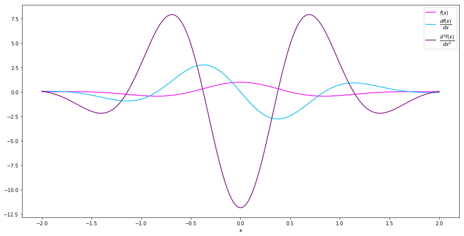
Both the methods evaluation_at and derivative_at are vectorized, and instead of pass in a scalar value, we can pass in a numpy.array, and the output will be f’s value / derivative at all entried of the input. For example, we can calculate the value, first order derivative and second order derivative of \(f(x)\) on the interval \([-2, 2]\) simply by

interval = np.linspace(-2, 2, 200)
values = f.evaluation_at(   {x: interval})
der1st = f.derivative_at(x, {x: interval})
der2nd = f.derivative_at(x, {x: interval}, order=2)

Let’s see what they look like.

fig  = plt.figure(figsize=(16, 8))
plt.plot(interval, values, c='magenta',     label='$f(x)$')
plt.plot(interval, der1st, c='deepskyblue', label='$\dfrac{df(x)}{dx}$')
plt.plot(interval, der2nd, c='purple',      label='$\dfrac{d^2f(x)}{dx^2}$')
plt.xlabel('x')
plt.legend()
plt.show()

Multivariate Functions

The workflow with multivariate functions are essentially the same.

Suppose we want to calculate the derivatives of \(g(x, y) = \cos(\pi x)\cos(\pi y)\exp(-x^2-y^2)\). We can start with adding another Variable called y.

y = Variable()

We then create the Expression for \(g(x, y)\).

g = cos(np.pi*x) * cos(np.pi*y) * exp(-x**2-y**2)

We can then evaluate \(f(x)\)‘s value and derivative by calling the evaluation_at method and the derivative_at method, as usual.

g.evaluation_at({x: 1.0, y: 1.0})

0.1353352832366127

g.derivative_at(x, {x: 1.0, y: 1.0})

-0.27067056647322535

g.derivative_at(x, {x: 1.0, y: 1.0})

-1.0650351405815222

Now we have two variables, we may want to calculate \(\dfrac{\partial^2 g}{\partial x \partial y}\). We can just replace the first argument of derivative_at to a tuple (x, y). In this case the third argument order=2 can be omitted, because the Expression can infer from the first argument that we are looking for a second order derivative.

g.derivative_at((x, y), {x: 1.0, y: 1.0})

0.5413411329464506

We can also ask g for its Hessian matrix. A numpy.array will be returned.

g.hessian_at({x: 1.0, y:1.0})

array([[-1.06503514,  0.54134113],
       [ 0.54134113, -1.06503514]])

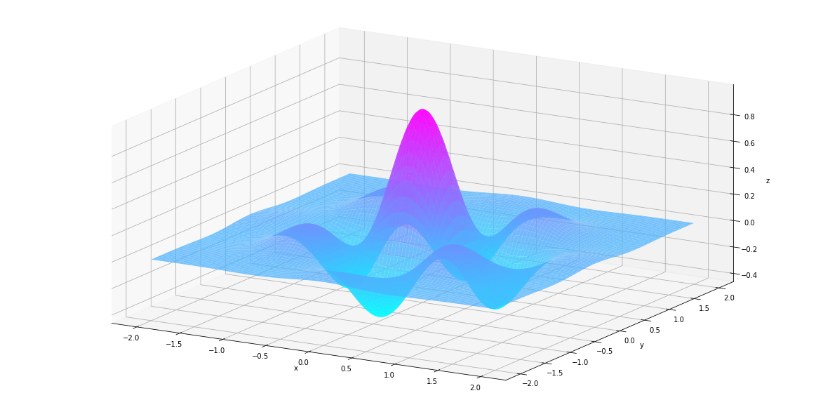
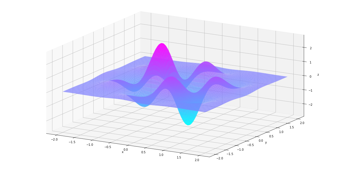
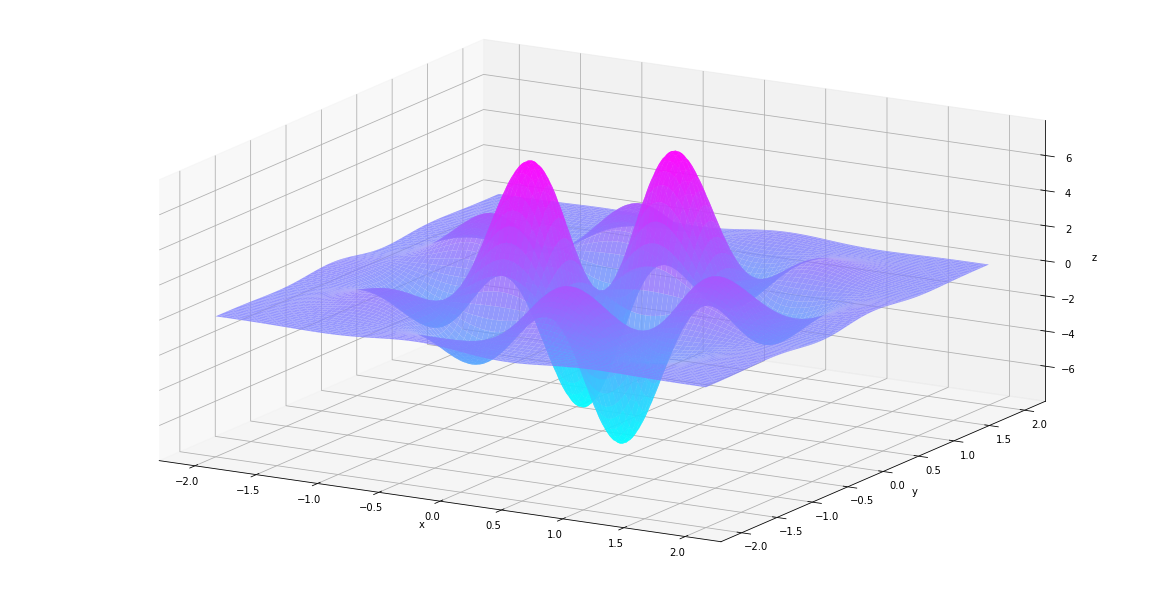
Since the evaluation_at method and derivarive_at method are vectorized, we can as well pass in a mesh grid, and the output will be a grid of the same shape. For example, we can calculate the value, first order derivative and second order derivative of f(x)f(x) on the interval \(x\in[−2,2], y\in[-2,2]\) simply by

us, vs = np.linspace(-2, 2, 200), np.linspace(-2, 2, 200)
uu, vv = np.meshgrid(us, vs)

values = g.evaluation_at(        {x: uu, y:vv})
der1st = g.derivative_at(x,      {x: uu, y:vv})
der2nd = g.derivative_at((x, y), {x: uu, y:vv})

Let’s see what they look like.

def plt_surf(uu, vv, zz):
    fig  = plt.figure(figsize=(16, 8))
    ax   = Axes3D(fig)
    surf = ax.plot_surface(uu, vv, zz, rstride=2, cstride=2, alpha=0.8, cmap='cool')
    ax.set_xlabel('x')
    ax.set_ylabel('y')
    ax.set_zlabel('z')
    ax.set_proj_type('ortho')
    plt.show()

plt_surf(uu, vv, values)

plt_surf(uu, vv, der1st)

plt_surf(uu, vv, der2nd)

Vector Functions

Functions defined on \(\mathbb{R}^n \mapsto \mathbb{R}^m\) are also supported. Here we create an VectorFunction that represents \(h(\begin{bmatrix}x\\y\end{bmatrix}) = \begin{bmatrix}f(x)\\g(x, y)\end{bmatrix}\).

h = VectorFunction(exprlist=[f, g])

We can then evaluates \(h(\begin{bmatrix}x\\y\end{bmatrix})\)‘s value and gradient (\(\begin{bmatrix}\dfrac{\partial f}{\partial x}\\\dfrac{\partial g}{\partial x}\end{bmatrix}\) and \(\begin{bmatrix}\dfrac{\partial f}{\partial y}\\\dfrac{\partial g}{\partial y}\end{bmatrix}\)) by calling its evaluation_at method and gradient_at method. The jacobian_at function returns the Jacobian matrix (\(\begin{bmatrix}\dfrac{\partial f}{\partial x} & \dfrac{\partial f}{\partial y} \\ \dfrac{\partial g}{\partial x} & \dfrac{\partial g}{\partial y} \end{bmatrix}\)).

h.evaluation_at({x: 1.0, y: -1.0})

array([-0.36787944,  0.13533528])

h.gradient_at(0, {x: 1.0, y: -1.0})

array([0., 0.])

h.jacobian_at({x: 1.0, y: -1.0})

array([[ 0.73575888,  0.        ],
       [-0.27067057,  0.27067057]])